The whole is greater than the sum of its parts
The whole is greater than the sum of its parts
Most modern scientific and engineering problems are complex systems. So what are those? Complex systems embody a profound and fascinating truth: the whole is greater than the sum of its parts. When we look at an individual atom, it appears deceptively simple - essentially a nucleus surrounded by electrons, governed by electromagnetic forces. Yet when atoms come together, they give rise to molecules, cells, organisms, ecosystems, societies, and civilizations. Each level of organization exhibits behaviors and properties that could not have been predicted by simply studying the components in isolation.
This emergence of complex behavior from simple rules is one of nature’s most remarkable features. Consider how a collection of neurons - each just a cell that fires electrical signals - somehow gives rise to consciousness and intelligence. Or how individual birds following basic flocking rules create mesmerizing aerial ballets that no single bird could choreograph.
One of the clearest demonstrations of this phenomenon comes from cellular automata - simple grid-based systems where each cell follows basic rules based on its neighbors’ states. The most famous example is Conway’s Game of Life, where cells live or die according to just four rules:
- Any live cell with fewer than two live neighbors dies (underpopulation)
- Any live cell with two or three live neighbors lives on to the next generation
- Any live cell with more than three live neighbors dies (overpopulation)
- Any dead cell with exactly three live neighbors becomes a live cell (reproduction)
From these simple rules emerge complex patterns and behaviors - gliders that move across the grid, oscillators that pulse in place, and even “guns” that periodically emit new patterns. This illustrates how complexity can emerge from simplicity through the interaction of basic components following basic rules.
Differential Equations: How local interactions describe global behavior
Our story begins with one of science’s most powerful tools: differential equations. Since Newton’s groundbreaking work in the 17th century, scientists have used these mathematical constructs to describe how things change locally in space and time. In its simplest and most abstract form, a differential equation is a relationship between a quantity \(x\) and its rate of change \(\dot{x}\) through an equation of the form:
\[\dot{x} = f(x, t)\]where \(f\) is some function of \(x\) and \(t\). The beauty of differential equations lies in their ability to capture the essence of physical phenomena through mathematical relationships between quantities and their rates of change at a given point in space and time. In other words, they show that both the future and past can be completely determined by how things are changing at a given point in space and time. This assumption is extremely powerful and has been used to great success in physics and engineering, but it comes with great limitations; particularly in complex systems.
Let’s look at some fundamental examples of differential equations that describe physical phenomena. We’ll start with linear equations and build up to nonlinear ones to understand how complexity emerges.
The heat equation in one dimension is one of the simplest partial differential equations:
\[\frac{\partial T}{\partial t} = \alpha \frac{\partial^2 T}{\partial x^2}\]where \(T(x,t)\) is the temperature at position \(x\) and time \(t\), and \(\alpha\) is the thermal diffusivity of the material. The left side represents how temperature changes with time, while the right side captures how heat flows from hot to cold regions. This linear equation tells us that heat naturally spreads out smoothly over time, always flowing from higher to lower temperatures.
 Visualization of heat diffusion in a material. The colors represent temperature, with red being hot and blue being cold. Notice how heat flows from hot to cold regions, smoothing out temperature differences over time.
The wave equation describes oscillating phenomena like sound waves or vibrating strings:
\[\frac{\partial^2 u}{\partial t^2} = c^2 \frac{\partial^2 u}{\partial x^2}\]where \(u(x,t)\) represents displacement and \(c\) is the wave speed. This equation shows how disturbances propagate through space at constant speed without changing shape. Again, it’s linear - doubling the initial disturbance doubles the response.
 Visualization of wave propagation in a medium. The colors represent displacement, with red being positive and blue being negative. Notice how the wave propagates through space at constant speed, maintaining its shape.
But nature isn’t always so well-behaved. The Navier-Stokes equations governing fluid flow introduce nonlinearity:
\[\rho(\frac{\partial \mathbf{v}}{\partial t} + \mathbf{v} \cdot \nabla\mathbf{v}) = -\nabla p + \mu\nabla^2\mathbf{v}\]Here ρ is density, v is velocity, p is pressure, and μ is viscosity. The nonlinear term v·∇v represents acceleration due to spatial changes in velocity. This seemingly innocent addition makes the equation extremely difficult to solve
- small changes in initial conditions can lead to dramatically different outcomes. This is why weather prediction becomes unreliable after a few days, and why smooth laminar flow can suddenly transition to turbulent chaos. Here’s an example of combustion in a turbulent mixing layer:
 The animations here show a numerical simulation of combustion in a turbulent mixing layer. The grayscale indicates density contours of a hydrogen-air mixture. The top layer is moving left to right, and the lower layer moves right to left. This sets up some very turbulent mixing, visible in middle as multi-scale eddies turning over on one another.
These are all common examples of systems that can be effectively modeled through the relationship between rates of change that are local in space and time. Are there any examples of systems that are not local in space and time?
Beyond Local Interactions: The Non-local Challenge
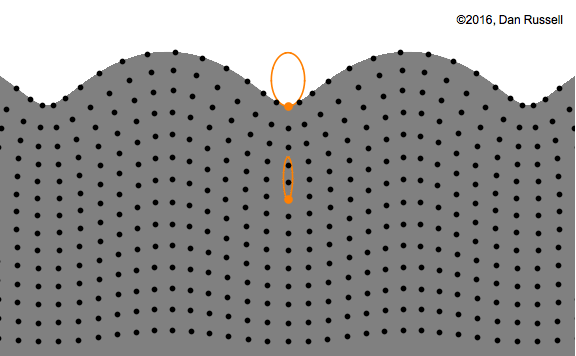
Nature isn’t always satisfied with local interactions. Many systems exhibit non-local effects, where changes in one region can instantly influence distant parts of the system. These phenomena require more sophisticated mathematical tools: integro-differential equations. These equations account for long-range interactions and memory effects, but they come at a cost. They are often difficult to derive from first principles and even harder to solve numerically. In its most basic form, a non-local equation is of the form:
\[\frac{d}{dt} x(t) = \int_{-\infty}^{\infty} K(t-s) x(s) ds\]where \(K(t-s)\) is the kernel function that describes the memory of the system.
Population dynamics with migration patterns, materials with memory effects, and quantum systems all exhibit non-local behaviors that challenge our mathematical frameworks. The complexity of these systems often forces us to make simplifying assumptions, potentially missing crucial aspects of the phenomena we study.
 This animation shows a crack propagating through a material. The crack is propagating through the material, and the voids are the regions where the material has been removed. The crack is propagating through the material, and the voids are the regions where the material has been removed. The crack is propagating through the material, and the voids are the regions where the material has been removed.
A Nonlinear and Chaotic World
Perhaps the most humbling aspect of complex systems is their inherent nonlinearity. Unlike linear systems, where effects are proportional to causes, nonlinear systems can exhibit dramatically disproportionate responses. This nonlinearity gives rise to chaos theory, exemplified by the famous “butterfly effect” – the notion that a butterfly flapping its wings in Brazil might cause a tornado in Texas.
Weather systems perfectly illustrate this challenge. Despite our sophisticated models and powerful computers, accurate weather prediction remains limited to a few days ahead. The chaotic nature of the atmosphere means that tiny uncertainties in our measurements grow exponentially over time, making long-term prediction fundamentally impossible.
The Multiscale Challenge
Most natural systems operate across multiple scales simultaneously. Consider a human body: from the molecular interactions in our cells to the coordinated action of organs, from individual neural firings to conscious thought, phenomena at each scale influence and are influenced by events at other scales. This multiscale nature presents a fundamental challenge to our understanding.
Similar challenges appear in climate science, where molecular processes must be connected to global patterns, or in materials science, where atomic interactions determine macroscopic properties. Our traditional models often struggle to bridge these scales effectively.
Complex Systems in Nature and Society
The examples of complex systems surround us:
-
Weather and Climate: Perhaps the most familiar complex system, where local atmospheric conditions interact to produce global weather patterns and long-term climate trends.
-
Active Matter: From schools of fish to flocks of birds, these systems demonstrate how simple interaction rules can produce complex collective behaviors.
-
Biological Systems: From cellular networks to ecosystems, living systems exhibit remarkable organization and adaptation.
-
Social Systems: Human societies, economies, and even artificial systems like social networks and Large Language Models demonstrate emergent behaviors that arise from countless individual interactions.
Modern Tools for Complex Challenges
To tackle these challenges, we’ve developed a powerful toolbox:
- Differential Equations: Still fundamental for describing local dynamics and forming the basis of many models.
- Probability and Statistics: Essential for handling uncertainty and extracting patterns from data.
- Scientific Computing: Enabling us to simulate complex systems and explore their behavior numerically.
- Machine Learning: Offering new ways to discover patterns and relationships in complex data.
The emergence of machine learning, particularly deep learning, offers new hope for understanding complex systems. Neural networks, with their ability to learn patterns from data without explicit programming, might help us discover relationships we never knew existed. As some researchers have suggested, “The next scientific discovery is hiding in a neural network.”
As we face these challenges, we must maintain the mindset of a scientist: embracing uncertainty, acknowledging what we don’t know, and approaching the world with wonder. Complex systems remind us of the vast frontiers of human knowledge still waiting to be explored.
The tools we’ve developed – from differential equations to machine learning – are not just mathematical constructs but windows into the nature of reality. Each new tool gives us a different perspective, and together they help us push the boundaries of our understanding.
The study of complex systems is more relevant than ever. As we face global challenges like climate change, pandemic response, and social inequality, we need tools that can handle complexity and uncertainty. The integration of traditional mathematical models with modern machine learning approaches offers new hope for understanding and managing these challenges.
The journey to understand complex systems is ongoing. Each answer reveals new questions, and each solution uncovers new challenges. But this is the nature of science – a continuous journey of discovery, guided by curiosity and enabled by our ever-expanding toolkit of mathematical and computational methods.