import numpy as np
import matplotlib.pyplot as plt
from matplotlib import rcParams
from scipy import io
import os
import matplotlib.cm as cm

rcParams.update({'font.size': 18})
plt.rcParams['figure.figsize'] = [8, 16]

## Building on Reference from: Data-driven Science and Engineering - Brunton and Kutz
results = io.loadmat(os.path.join('cyl_flow_data.mat'))
vortmean = np.mean(results['VORTALL'], axis=1)
X = results['VORTALL'] - vortmean.reshape((-1,1))

# VORTALL contains flow fields reshaped into column vectors

def DMD(X,Xprime,r):
    # Step 1: SVD of X
    U,Sigma,VT = np.linalg.svd(X,full_matrices=0)
    Ur = U[:,:r]
    Sigmar = np.diag(Sigma[:r])
    VTr = VT[:r,:]

    # Step 2: Compute Atilde
    Atilde = np.linalg.solve(Sigmar.T,(Ur.T @ Xprime @ VTr.T).T).T

    # Step 3: Compute eigenvalues and eigenvectors
    Lambda, W = np.linalg.eig(Atilde)
    
    # Step 4: Compute Phi
    Phi = Xprime @ np.linalg.solve(Sigmar.T,VTr).T @ W
    alpha1 = Sigmar @ VTr[:,0]
    b = np.linalg.solve(W @ np.diag(Lambda),alpha1)
    return Phi, Lambda, b

Phi, Lambda, b = DMD(X[:,:-1],X[:,1:],21)

# Reconstruct system dynamics (inference)
timesteps = X.shape[1]
time_dynamics = np.zeros((21, timesteps), dtype='complex')

for i in range(timesteps):
    time_dynamics[:, i] = b * (Lambda ** i)  # Element-wise exponential growth

X_dmd = Phi @ time_dynamics  # Reconstructed data

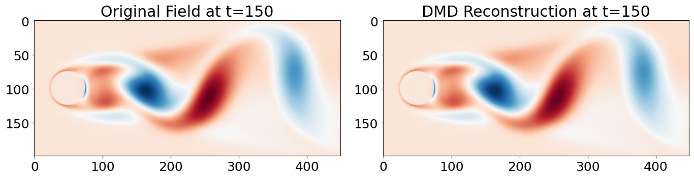
# Compare original and reconstructed at selected frame
frame_idx = 150  # Choose any time index < timesteps

original_field = np.real(np.reshape(X[:, frame_idx], (449,199))).T
reconstructed_field = np.real(np.reshape(X_dmd[:, frame_idx], (449,199))).T

vmin = min(original_field.min(), reconstructed_field.min())
vmax = max(original_field.max(), reconstructed_field.max())

fig, axes = plt.subplots(1, 2, figsize=(14, 6))
axes[0].imshow(original_field, cmap=cm.RdBu, vmin=vmin, vmax=vmax)
axes[0].set_title(f'Original Field at t={frame_idx}')

axes[1].imshow(reconstructed_field, cmap=cm.RdBu, vmin=vmin, vmax=vmax)
axes[1].set_title(f'DMD Reconstruction at t={frame_idx}')

plt.tight_layout()
plt.show()

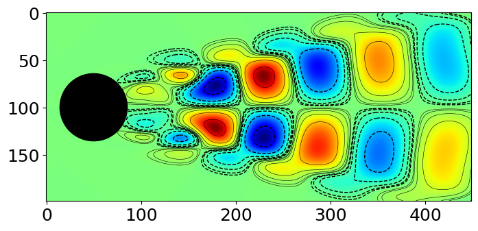
## Plot Mode 2
vortmin = -5
vortmax = 5
V2 = np.copy(np.real(np.reshape(Phi[:,9],(449,199))))
V2 = V2.T

# normalize values... not symmetric
minval = np.min(V2)
maxval = np.max(V2)

if np.abs(minval) < 5 and np.abs(maxval) < 5:
    if np.abs(minval) > np.abs(maxval):
        vortmax = maxval
        vortmin = -maxval
    else:
        vortmin = minval
        vortmax = -minval

V2[V2 > vortmax] = vortmax
V2[V2 < vortmin] = vortmin

plt.imshow(V2,cmap='jet',vmin=vortmin,vmax=vortmax)

cvals = np.array([-4,-2,-1,-0.5,-0.25,-0.155])
plt.contour(V2,cvals*vortmax/5,colors='k',linestyles='dashed',linewidths=1)
plt.contour(V2,np.flip(-cvals)*vortmax/5,colors='k',linestyles='solid',linewidths=0.4)

plt.scatter(49,99,5000,color='k') # draw cylinder


plt.show()